Blog

Let’s recall the functions we learned in the first week of the course.

Cost function

$$ J(\theta_0, \theta_1) = \frac{1}{2m} \sum_{i=1}^{m} (h_\theta(x^{(i)}) - y^{(i)})^2 $$

This is the function to tell us how far our line defined by $h_\theta(x) = \theta_0 + \theta_1x$ is from the cloud of dots with the training set plotted. $m$, in the function, represents the number of training examples we have available, while x the variable and y the answer for each example. So, $x^{(2)}$ is the value of the first feature in the second example.

Gradient Descent algorithm

$$ \theta_0 := \theta_0 - \alpha\frac{\partial}{\partial\theta_j} J(\theta_0, \theta_1) $$ $$ \theta_1 := \theta_1 - \alpha\frac{\partial}{\partial\theta_j} J(\theta_0, \theta_1) $$

or after calculating the derivative:

$$ \theta_0 := \theta_0 - \alpha\frac{1}{m} \sum_{i=1}^{m} (h_\theta(x^{(i)}) - y^{(i)}) $$ $$ \theta_1 := \theta_1 - \alpha\frac{1}{m} \sum_{i=1}^{m} (h_\theta(x^{(i)}) - y^{(i)})x^{(i)} $$

Gradient Descent is the responsible to converge values of $\theta_0$ and $\theta_1$ until reaching the best line possible to define the dots graph.

Taking It To The Next Level

This second week we start learning the variation of Linear Regression called “Multivariate linear regression”. They probably had a good reason to name it like this…

When analysing a dataset of house sales, we surely can predict the price for a given property checking how others with the same size perform. But after knowing a little more about the market, it is obvious that these prices aren’t defined by just their size. Checking for the relationship between size, number of floors, age, number of bedrooms may return more trustworthy results. For accomplish this goal, we have expand previously showed equations to accommodate multiple features.

The known cost function changes from

$$ h_\theta(x) = \theta_0 + \theta_1x $$

to

$$ h_\theta(x) = \theta_0 + \theta_1x_1 + \theta_2x_2 + \theta_3x_3 + … + \theta_nx_n $$

In the end, everything stays in the same place. The function will still form a line, but from now on will depend over multiple values - the x’s. $\theta$’s still correspond to the numbers responsible for moving this line nearest as possible of the dots.

The gradient descent algorithm has a version supporting multiple features.

$$ \theta_0 := \theta_0 - \alpha\frac{1}{m} \sum_{i=1}^{m} (h_\theta(x^{(i)}) - y^{(i)}) $$ $$ \theta_1 := \theta_1 - \alpha\frac{1}{m} \sum_{i=1}^{m} (h_\theta(x^{(i)}) - y^{(i)})x^{(i)} $$

changes to

$$ \theta_0 := \theta_0 - \alpha\frac{1}{m} \sum_{i=1}^{m} (h_\theta(x^{(i)}) - y^{(i)})x_0^{(i)} $$ $$ \theta_1 := \theta_1 - \alpha\frac{1}{m} \sum_{i=1}^{m} (h_\theta(x^{(i)}) - y^{(i)})x_1^{(i)} $$ $$ \theta_2 := \theta_2 - \alpha\frac{1}{m} \sum_{i=1}^{m} (h_\theta(x^{(i)}) - y^{(i)})x_2^{(i)} $$

…

Consider $x_0^{(i)} = 1$ and gradient descent also stays the same for the first two features.

Some Tricks

OK, every function and algorithm learned will result in the right values. But depending on how your dataset is, this may take a lot of time. Andrew Ng in some videos of this week teach us how to accelerate this process.

The first trick is feature scaling. Having features in different scales - for instance, house area in something around 2000 and number of bathrooms between 1 and 5 - cause gradient descent calculations to take a lot of time.

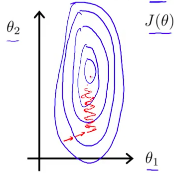
Imagine the center of all circles the position where best values for $\theta$ stays and each red arrow as an iteration of the algorithm.

It’s time to use feature scaling - dividing each feature by its range. If bathrooms are in a range of 1 and 5, divide all values in the dataset by 4. For areas ranging between 1000 and 3000, divide them by 2000.

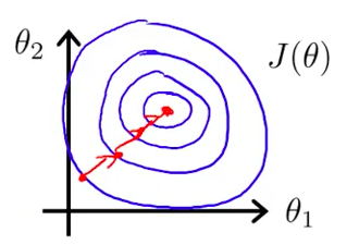
This is the result after feature scaling.

Doing so will require less iterations to reach the goal.

Another smart trick is “approximating” the graph from the point (0,0) of the graph. Since the arrows start on that point, would be way faster to reach anything near. For this, subtract the mean feature value from each value before the scaling.

$$ X_1 := \frac{X_1 - \mu_1}{S_1} $$

This mathematical representation shows what happens with the feature $X_1$ after normalization. It’s subtracted by its mean and divided by standard deviation (the beautiful name for that range of available values). You just need to remember to denormalize the value you discover after receiving a result from the algorithm. In other words, you must do the reverse operation, multiplying by standard deviation and adding mean.

The key rule is knowing your data and experimenting. Sometimes you may have a database with duplicated features - house age and date of its construction -, something that may be simplified - “frontage” and “depth” becoming a single feature called “size” - or just something that can return the same result faster if you give a smaller learning rate (the α in the gradient descent).

A Touch Of Linear Algebra

Hey, don’t leave me already! There’s no big deal about Linear Algebra. The course provides a good review (of 1 hour) about the subject, and if you don’t know why the hell a matrix may be useful to solve equations like the ones we have here, watch this lecture from Professor Gilbert Strang.

The same results are reachable even without the gradient descent algorithm. For small datasets, the Linear Algebra solution can give you faster results.

$$ \theta = (X^T X)^{-1}X^T y $$

In this equation, each value is a matrix. $\theta$ contains all values for theta, while $X$ the entire feature dataset and y, existing results (for the housing price problem, would be a price matrix).

Octave

This is the tool suggested to be used for calculating results by implementing algorithms. The week lectures include videos about Octave and how to use it to perform calculations using matrices, iterations, assignments and graph plotting.

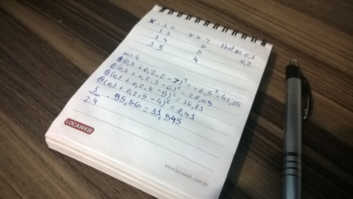
Being honest, I thought that would be easy and just a matter of a couple of hours to send all the assignments. Solving the exercises, in the end, took me an entire day. Forcing myself to use iterative processes - while studying functional programming for a good time - as recommended by the course messed a little with my head. The solution was to take a piece of paper and write the result I expected and debug my wrong solution.

It was enough to read two datasets with multiple features, using matrices as much as possible. Mission accomplished!